Sven Thiele 0000-0002-5812-6963
· sthiele
Analysis and Redesign of Biological Networks, Max Planck Institute for Dynamics of Complex Technical Systems Magdeburg
Axel von Kamp
· axelvonkamp
Analysis and Redesign of Biological Networks, Max Planck Institute for Dynamics of Complex Technical Systems Magdeburg
Pavlos Stephanos Bekiaris 0000-0002-3047-4253
· Paulocracy
· Paulocracy2
Analysis and Redesign of Biological Networks, Max Planck Institute for Dynamics of Complex Technical Systems Magdeburg
Philipp Schneider
· VonAlphaBisZulu
Analysis and Redesign of Biological Networks, Max Planck Institute for Dynamics of Complex Technical Systems Magdeburg
Introduction
Welcome to CNApy’s user manual!
CNApy [Paper] is a Python-based graphical user interface for a) many common methods of Constraint-Based Reconstruction and Analysis (COBRA) with stoichiometric metabolic models, b) the visualization of COBRA calculation results as interactive and editable metabolic maps (including Escher maps [GitHub][Paper]) and c) the creation and editing of metabolic models, including its reactions, metabolites and genes. For model loading and export, CNApy supports the widely used SBML standard format [Site][Paper].
Supported COBRA methods (partly provided by cobrapy [GitHub][Paper]) include:
Thermodynamic methods based on OptMDFpathway [Paper]
Many advanced strain design algorithms such as OptKnock [Paper], RobustKnock [Paper], OptCouple [Paper] and advanced Minimal Cut Sets [Paper] through its StrainDesign [GitHub][Paper] integration
We appreciate any comments or suggestions for improvements and we are greatly interested in your feedback! If you have questions, suggestions or bug reports regarding CNApy, you can use either of the CNApy GitHub issues, the CNApy GitHub discussions or the CNApy Gitter chat room.
Thank you for using CNApy!
Installation
CNApy main program
There are 4 alternative ways to install CNApy:
The easiest way for any user to install CNApy is by downloading its installer, which is provided for Windows, Linux and MacOS, see Using CNApy installer for more.
If you already have installed Python 3.10 (no other version) on your system, you can install CNApy simply through pip install cnapy in your console. Afterwards, you can start CNApy’s GUI by running either cnapy or, if this doesn’t work, python -m cnapy where “python” must call your Python 3.10 installation.
If you already use conda or mamba (for mamba, just change the “conda” command to “mamba”), you can create a CNApy environment named cnapy-1.2.2 as follows: 1) Run conda create --name cnapy-1.2.2 python=3.10 pip openjdk -c conda-forge, 2) run conda activate cnapy-1.2.2, 3) run pip install cnapy. Then, you can start CNApy in the cnapy-1.2.2 conda environment by running either cnapy or, if this doesn’t work, python -m cnapy. Note that the cnapy conda package is currently not being updated due to licensing uncertainties.
If you want to develop CNApy, follow the instruction for the cloning and setup of the CNApy repository using git and conda or mamba in section Setup the CNApy development environment.
Note: After CNApy’s installation, it is recommended to download the CNApy example projects (including interactive maps of models such as ECC2, iML1515 and many more) by starting CNApy and clicking on “Download CNApy example projects…” in the “Projects” menu entry or by following the first start-up instructions.
Installing additional solvers (optional)
CNApy itself is already packaged and installed with the open source linear programming solver GLPK which is fast enough for simple calculations with small models and which is not restricted in the possible number of variables.
For strain design and thermodyanmic calculations, you can also use the free and open-source solver SCIP which is much faster than GLPK but still often much slower than IBM CPLEX and Gurobi (see next paragraph). You can install SCIP by following the instructions on its website.
In addition, CNApy comes pre-packaged with the Community editions of the much faster commercial solvers IBM CPLEX and Gurobi. These community editions can only run with models up to 1000 variables. In order to use one of these solvers with models which contain more variables, the full versions of either two of these solvers have to be installed and connected to CNApy. You can obtain these full versions from CPLEX’s and Gurobi’s web sites, respectively.
In order to help you with the installation of the full versions, CNApy contains a wizard which explains the process in detail and which takes over some of the neccessary tasks. You can find these wizards under the “Config” menu entry. Click on the wizard menu entry, and follow the wizard’s detailed instructions.
Configuration
CNApy can be configured via the Config menu. The different aspects of CNApy can be configured via separate dialogs:
Configure CNApy
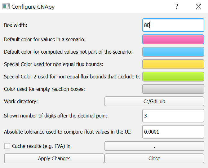
Figure 1:CNApy Configuration dialog.
Here you can configure which colors CNApy should use to highlight reactions on the map or in the reaction list.
In addition, you can activate the flux analysis (e.g., flux variabiliy analysis or FVA) cache in the selected folder, where flux analysis results of a specific model will be stored so that they can be quickly reloaded without performing the flux analysis again. The flux analysis cache automatically works in a way such that any change of the model also leads to a newly created flux analysis cache file.
Configure COBRApy
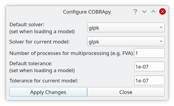
Figure 2:COBRApy configuration dialog.
With this dialog selected global settings (class cobra.Configuration()) of the COBRApy toolbox and selected parameters of the current model can be modified. The global settings are saved, but the parameters of the current model are not and will revert to the global default values when (re-)loading a model.
Default solver (global)
Select which solver to use as global default from the dropdown list. COBRApy supports a variety of solvers but only the ones which are installed for COBRApy on your system will be available on the list. Also, different solvers have different capabilities so you should set a default that has all capabilities that you require (e.g. glpk_exact cannot be used for MILPs).
Solver for current model
Here you can change the solver for the current model.
Number of processes for multiprocessing (global)
Number of processes run in parallel when Python multiprocessing is used, e.g. for FVA. Setting this to 1 disables multiprocessing.
IMPORTANT
Should be set to 1 on Windows because Python multiprocessing performs very poorly on this OS.
Default tolerance (global)
This value is used to distinguish zero from non-zero elements for various purposes. In particular, this value is propagated to the solver (see the COBRApy source code which solver parameters are affected). Most solvers restrict the range of this value, so it must be between 1E-9 and 0.1 For details where this value is used see the COBRApy documentation and source code.
Tolerance for the current model
Here you can change the tolerance for the current model. You may enter an arbitrary value >= 0 here but if it is not compatible with the current solver then “Apply Changes” can lead to an error message.
User interface overview
This section gives an introduction to the CNApy UI and its components and functions.
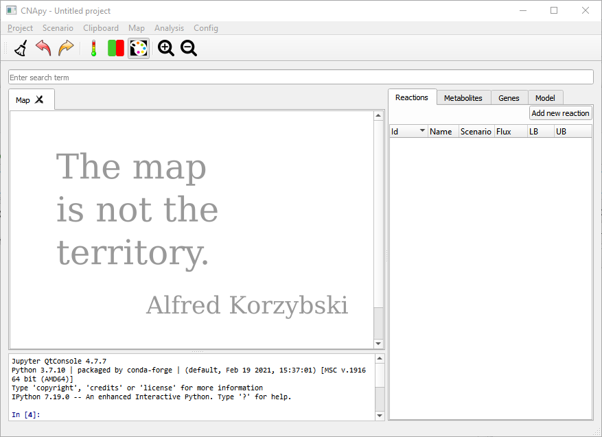
Figure 3:CNApy with an empty project.
This is an empty project on the right hand side we see the empty lists of reactions, metabolites and genes.
On the left we see the embedded Jupyter Console where one can interact programmatically with the model and UI.
We can create a new project by importing SBML models, editing the reactions and adding graphical maps.
We can also load one of the projects included in our projects repository.
Let’s go to Project in our menubar and open the ECC2comp.cna project.
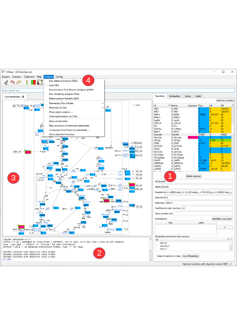
Figure 4:CNApy with the ECC2comp project.
In this picture we see CNApy with the open ECC2comp project.
On the right hand side (1) we see the populated reactions and metabolites lists with the color coded current values and a form with corresponding details for the selected reaction/metabolite.
The upper part of the reactions lists contains several columns. In the “Scenario” column the current scenario values are shown and can also be edited via this column. The “Flux” column contains the results of the last computation, e.g. the fluxes from a FBA. The “LB” and “UB” columns show the lower/upper bounds of the reactions and after a FVA the results of this analysis will be displayed there.
The reactions list contains buttons that lets us add/delete reactions to/from the model.
Changing the metabolite identifier or other details in the metabolite/reaction form has an instant effect on the corresponding reactions/metabolites in the model.
When selecting a metabolite in the metabolite tabs a list of reactions (and corresponding equations) in which this metabolite participates is shown a the bottom. By double-clicking on a reaction or metabolite ID one can switch to the respective object.
The console (2) now shows the output of some computations, and above the console we have a map view (3) with a graphical representation of our network.
On top (4) we have the menu bar which gives us access to the various functionalities of CNApy and a Toolbar for quick access to often used functions.
Underneath, you can also see the search bar with which you can search for the IDs of reactions, metabolites or genes, depending on which tab you have opened. The search results are shown in the respective list (1). In addition to only searching for IDs, you can also look for annotations (given in the annotations table of a single reaction, metabolite or gene) if you activate the respective checkbox.
We can add new maps via the Map menu, and drag reactions from the reaction list onto the desired position on the map.
Create a new project
In this section we explain how to create a new metabolic network project.
We also have a video on that topic https://youtu.be/bsNXZBmtyWw.
CNApy starts with an empty project.
You can directly add new reactions via the reaction mask on the right.
by pressing the Add new reaction button.
Then, you can type the reaction formula into the Equation field. For example A + 2 B -> C.
The associated metabolites A, B and C are then automatically added to the model.
Changing metabolite identifiers in the metabolite form instantly rewrites the reaction equation of the associated reactions.
Since creating big models by adding single reactions is very cumbersome, CNApy also allows you to create a new project from a pre-existing SBML file.
You find the action New project from SBML in the Project menu.
After importing an SBML model, the reaction list is populated with all the reactions from the model.
You can add a map to the project by going to the Map menu and clicking add new map.
From the Map menu we can also change the background image of our map.
Any SVG image can be used as a background.
You can add multiple maps that highlight different aspects of your model.
Reaction boxes can be put on the map by dragging over them from the reactions list.
You can adjust the box size with the keyboard shortcuts Ctrl + + and Ctrl + -.
You can move the reaction box to the desired position by dragging them on their handles.
If you want to move all reaction boxes together, press Ctrl while dragging.
You can also set a specific (pixel-wise) position by right-clicking on a reaction box and selecting “set box position…”.
Positioning a big number of reaction boxes can be tiresome.
Therefore, CNApy allows you to load and save reaction box positions via the Map menu.
This facilitates reuse among similar projects.
The size of the background image can be adjusted with the shortcuts Ctrl + Shift + + and Ctrl + Shift + -.
To save a project click Save Project as in the Project menu.
It is important to add the .cna extension to the file name.
This way your files can be directly found by CNApy. .cna files both include the metabolic model as well as its associated maps.
Scenarios
In CNApy you can define a scenario under which metabolic analyses like the FBA will be performed.
In its most basic form, a scenario is a set of flux bounds for a set of reactions. A scenario flux can fix the flux of a reaction or set a lower and upper bound for the flux.
Furthermore, a scenario can contain its own objective function and it is possible to add reactions as well as constraints over the reaction fluxes to a model.
Scenario fluxes
The scenario fluxes of regular model reactions can be edited via the reaction boxes on the map or the Scenario column of the reaction list.
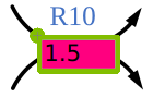
Accepted values are either a single float like 1.5 or a pair of floats like -10, 1.2.
A single float fixes the flux of the reaction to this value (1.5) while a pair sets the lower flux bound of the reaction to the first value (-10) and the upper flux bound to the second value (1.2).
Note that in a scenario you can use values outside the defined lower/upper bound of a reaction. In such a case the scenario will supersede the reaction bounds which allows temporary modification of the bounds without the need to change the model.
Figure 5:Reaction box with scenario value.
Reactions boxes with scenario flux are marked by the scenario color and a green frame.
The frame turns yellow, if the scenario flux lies outside the reaction bounds of the model.
To remove a scenario flux, simply delete the scenario value in the reaction box or “Scenario” column of the reaction list.
The Scenario tab
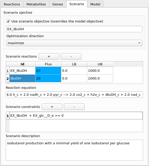
Figure 6:Scenario tab with settings for isobutanol production.
Scenario objective
A scenario objective can be defined in the Scenario tab. There it is also possible to select whether the scenario objective or the model objective is to be used (e.g. in FBA).
Scenario reactions
Scenario reactions can be added via the scenario tab. All metabolites from the model can be used when entering a reaction equation. If you use a metabolite that is not part of the model it will automatically be added to the model whenever the scenario is applied (e.g. in FBA). Scenario reactions are intended as a means for introducing a few reactions that are necessary for a scenario’s function without having to modify the model. Note that is not possible to set further properties of scenario reactions (e.g. a gene rule) or metabolites (e.g. a formula). If this is required then you need to add the respective reaction or metabolite to the model itself.
Scenario constraints
These are linear (in-)equality constraints over the reaction fluxes in the network (model as well as scenario reactions). Such a constraint can for instance be used to express a minimal product yield that is required in the scenario.
Scenario files and history
You can save and load scenarios as *.scen files via the Scenario menu or the toolbar. If a scenario file has been loaded its name is shown in the toolbar.
The flux bounds of a scenario can be set as the default scenario of your project.
This can be done via set current scenario as default scenario in the Scenario menu.
The project must then be saved, and the next time you open the project the scenario is already set.
CNApy implements an edit history for the scenario fluxes and with the tool buttons you can undo/redo your changes. Note that the edit history is for scenario fluxes only, scenario reactions and constraints can only be added/removed via the Scenario tab.
You can also import all the values that are currently in the reaction boxes into the scenario (can be useful for applying a MCS), and you can change the model’s reaction bounds to the current scenario flux values.
Analysis functions
Flux balance analysis (FBA)
Optimizes the value of the current objective function and shows a flux distribution that realizes this optimum.
The objective function is a linear function over the reaction rates in the network, its coefficients can be modified in the reaction dialogs.
To display the current objective function you can choose Show optimization function from the Analysis menu.
The current objective value is shown in the console as well as the status bar at the bottom of the main window.
Note that the flux distribution calculated by FBA is usually not unique.
Auto FBA
This is a checkable option which switches the “Auto FBA” mode on or off. In “Auto FBA” mode a FBA is automatically performed when a scenario is changed or when a reaction property that potentially influences the FBA result is changed.
Parsimonious FBA (pFBA)
In parsimonious FBA first the objective function optimized and then with this optimum as additional constraint the sum of the fluxes in the network is minimized.
This has the advantage that redundant internal cyclic fluxes are suppressed and that a lot of reactions will have zero flux which makes the solution easier to understand.
Flux variability analysis (FVA)
In FVA the maximal/minimal rate of each reaction is calculated.
This gives the possible flux range for each reaction.
Make scenario feasible
A scenario is infeasible if the given fluxes in this scenario are incompatible with each other. An example would be a flux of a product that is higher than the substrate flux multiplied by the maximal product yield. Such a situation could for instance arise due to measurement errors if the given fluxes come from experimental measurements.
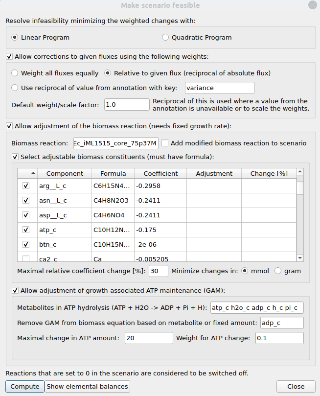
With “Make scenario feasible” the given fluxes in the scenario and/or the biomass composition are adjusted to make the fluxes consistent. This basically relies on minimzing the sum of deviations from the given fluxes and/or deviations from the stoichiometric coefficients the biomass reaction. There is one main setting that controls this minimization: One can choose whether the deviations are linear or quadratic terms, resulting in a linear program (LP) or quadratic program (QP) respectively (the latter requires a QP-capable solver like CPLEX or Gurobi).
Figure 7:Make scenario feasible dialog.
Allow corrections to given fluxes using the following weights
If this option is activated, adjustments of the given fluxes are allowed. Here you can set the (reciprocal) weights with which the flux deviations enter the objective function: They can either all be equal, relative to their absolute flux values (i.e. larger fluxes are more likely to be changed when resolving infeasibility), or taken from a specified field in the reaction annotation. In the last case, where a reaction has no entry in the specified annotation field, the default weight is used. The default weight/scale factor also scales all flux deviation weights and can thus be used to adjust the relative importance between flux corrections and biomass adjustments in the minimization. Concretely, lowering the scale factor here means that flux deviations become more expensive than biomass adjustments.
Allow adjustment of the biomass reaction
If this option is activated the biomass composition may be changed during minimization. To use this option it is required to selecet a biomass reaction and this reaction must have a fixed flux in the current scenario. There are two major ways in which the biomass reaction can be modified: The biomass composition may be allowed to change and/or the amount of growth-associated maintenance (GAM) may vary.
Select adjustable biomass constituents
Here a table is shown with the components of the biomass reactions as well as their stoichiometries and formulas. In the first column of this table you can (de-)select the components whose stoichiometries may be allowed to change. Note that you can only select components that have a formula so that their molecular weights can be calculated. These are required to set up a constraint which ensures that the overall biomass weight remains constant. You can also specify the maximal relative coefficient change [%] and whether the change should be calculated in mmol or gram.
Allow adjustment of growth-associated ATP maintenance (GAM)
If GAM is integrated in the currently selected biomass reaction this option can be used to activate the adjustment of GAM. For this you need to specify a list of metabolites of an ATP hydrolysis reaction together with the amount of GAM that has been set in the model. The GAM amount can either be given as a number or you can specify a metabolite of the ATP hydrolysis reaction (ADP should work in most situations) whose coefficient from the biomass reaction is then used as GAM amount. If all the above parameters are set, GAM will be removed from the biomass reaction during minimzation and considered separately. Lastly, you can set the maximal amount of GAM change together with a weight for this change in the overall minimization.
Compute
After optimization, the current scenario is modified so that it contains the calculated consistent fluxes and the necessary changes are shown on the console. If any adjustment of the biomass reaction occured then the modified biomass reaction is also shown on the console and it is added to the current scenario (see Scenario tab) if the “Add modified biomass reaction to scenario” was activated. The biomass and GAM adjustment results are also displayed in the dialog window. You can perform the calculation repeatedly with different settings while the dialog is open without the need to go back in the scenario history. You can reset the original scenario fluxes via the scenario history, but if a modified biomass reaction was added to the scenario you need to remove this via the Scenario tab.
Note that only reactions with scenario fluxes fixed to values unequal to zero enter the optimization. Reactions which have a zero flux set in the scenario will be considered removed from the network.
Known issue: The solvers are currently accessed through the optlang interface. Setting up the quadratic ojective for the QP via this interface incurs a significant overhead which increases with the number of fluxes set in the scenario. This means that the method as a whole can become quite slow in case more than a few dozen fluxes were set despite the fact that solving the QP itself is ususally quite fast.
Show elemental balances
Computes the elemental balances over
1) the boundary reactions with a given scenario flux
2) all boundary reactions with a computed flux.
If a biomass reaction is currently selected it is also included in the calculation. The results are then displayed on the console.
Note that this function only gives correct results if all metabolites included in the reactions have correct formulas.
Elementary modes (EFM)
EFM can be calculated via efmtool which is automatically installed with CNApy. After calculation a navigation panel appears to acces the results.
Options
When reactions are marked with 0 flux in a scenario and the option “consider 0 in current scenario as off” is activated then only the subset of EFM/EFV is calculated in which these reactions do not participate
Computational strain design
Minimal cut sets
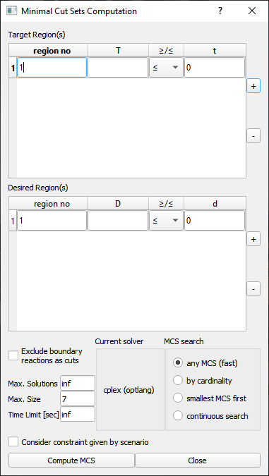
Minimal cut sets (MCS) can be calculated in CNApy using the dual method. After calculation a navigation panel appears to acces the results.
Figure 8:Minimal cut sets computation dialog.
Target and Desired region(s)
For the dual method one or more target regions must be defined which describe the network behaviour that is to be suppressed.
In addition, one or more desired regions may be defined which describe the network behaviour that is to be preserved.
Each target/desired region is defined by a set of linear equality constraints over the reaction rates in the network.
All target and desired regions must be initially feasible or an error will be raised. Also make sure that 0 is not included in any target or desired region (0 as target cannot be suppressed and 0 as desired is always fulfilled).
Note that all non-default reaction bounds (as defined by cobra.Configuration().bounds) are automatically added to all target and desired regions before MCS computation.
Current solver
MCS can be calculated via optlang using the currently active MILP solver.
Not all variants and solvers allow for the same options so these will partly be disabled depending on the chosen solver.
Max. solutions
Maximal number of MCS to calculate.
Max. size
Only calculate MCS which consists of up to this number of cuts.
Time limit
Do not run the search for longer than this limit.
It is strongly recommended to use this parameter because MCS computation can take very long especially when searching for smallest MCS.
MCS search
MCS can be enumerated iteratively, either the smallest first (least number of cuts) or any MCS (up to the number of cuts given by max. size).
With the latter option new MCS are found more quickly but may not be the smallest.
With CPLEX or Gurobi as solver, MCS can also be enumerated by cardinality, i.e. all MCS of successively increasing size (up to max. size) are computed.
In addition, with these solvers a continuous search mode is possible which is similar to the any MCS method but usually much faster.
Exclude boundary reactions as cuts
Do not allow knock-out of boundary reactions (reactions that cross the system boundary, e.g. exchange reactions).
Consider constraints given by scenario
Take reaction bounds set by the current scenario into account for all target and desired regions.
Compute strain designs
Opens a dialog which serves as front-end of the StrainDesign package for MILP-based strain design computation which supports MCS, MCS with nested optimization, OptKnock, RobustKnock and OptCouple, GPR-rule integration, gene and reaction knockouts and additions as well as regulatory interventions. A detailed description can be found in its documentation.
EFM/MCS Navigation and analysis
After the computation of EFM or MCS a navigation panel appears below the map. With this you can browse through the results, select a subset of the modes/MCS and show some statistics. There is also a button for saving the results and one to clear them and close the navigation panel.
Figure 9:Mode/MCS Navigation Panel.
Select…
In this text field you can enter a comma-separated list of reaction IDs. After pressing “Enter” on the keyboard the subset of modes/MCS is shown in which all specified reactions occur. If you prepend a reaction ID with an exclamation mark (e.g. !R1) this means that the specified reaction must not participate in selected the modes/MCS. To revert the selection click on the clear button embedded in the text field.
Reaction participation
Calculate the relative participation of each reaction in the currently selected modes/MCS. The results are shown in the reaction boxes and the “Flux” column of the reaction list.
Size histogram
Calculate the pathway lengths/number of reactions of the currently selected modes/MCS. The result is shown as a size historam in the integrated Jupyter console.
Flux optimization
Launches a dialog in which you can enter a linear expression (over the fluxes) that can then be maximized or minimized. The result is then displayed on the map(s) and the reaction list.
The flux values of the current scenario are taken into during the optimization.
Yield optimization
Launches a dialog in which you can enter two linear expressions (over the fluxes), which serve as numerator/denominator of a linear-fractional program which is then maximized or minimized.
A typical application would be the maximization of a product yield: When the exchange fluxes for ethanol and glucose are EX_etoh and EX_glc then maximizing EX_etoh/-EX_glc gives the maximal ethanol yield on glucose.
For this to work correctly, there must be no flux vector in the network where the denominator becomes zero and the nominator is non-zero.
The result is then displayed on the map(s) and the reaction list.
The flux values of the current scenario are taken into during the optimization.
Plot flux space
Launches a dialog in which you can configure a plot that shows the projection of the solution space in 2D or 3D where the axes can be flux expressions or yield expressions.
In the simplest case one can for example plot the growth rate against the substrate uptake rate.
The flux values of the current scenario are taken into account during the calculations.
OptMDFpathway
Launches a dialog with which you can start OptMDFpathway, a mixed-integer linear program which allows one to find - with a given metabolic network, linear constraints (such as a minimal growth rate), metabolite concentration ranges and Gibbs free energies of reactions (ΔG’°) - a pathway with the highest possible max-min driving force (MDF, in kJ/mol). If the MDF is negative, one knows that, at least as deduced by the given thermodynamic data (metabolite concentration ranges and Gibbs free energies), there is no thermodynamically feasible solution. If the MDF is positive, one knows that there is a thermodynamically feasible solution.
In order to set-up a CNApy model for OptMDFpathway (or any of the following thermodynamics-using methods), you have to provide metabolite concentration ranges as well as reaction ΔG’° values as mentioned below.
Once this is set up, you can run OptMDFpathway either at the optimal value of the model’s or scenario’s objective (which is calculated in advance without thermodynamic constraints) by activating the checkbox, or without regarding the objective value.
Thermodynamic FBA
This thermodynamic FBA is derived from OptMDFpathway (see above) and requires a minimal MDF that must be at least reached and for which a steady-state solution is searched for. The main difference to OptMDFPathway is that the given steady-state solution does not have to be at the OptMDF, but just at any MDF between the given minimal MDF and the OptMDF, which allows for more possible solutions. E.g., if you set a small positive minimal MDF of, e.g., 0.0001 kJ/mol, you essentially perform an FBA where thermodynamic feasibility is ensured. Again, if you activate the checkbox, you can perform this calculation at the optimal objective value which is calculate in advance.
Note that, just like with normal flux balance analysis and OptMDFpathway, the resulting flux solution does not have to be unique.
Thermodynamic bottleneck analysis
Each thermodynamic solution is restricted by at least one thermodynamic bottleneck, i.e., there is at least one reactions whose ΔG’° poses a limit on the OptMDF with the given metabolite concentration ranges. In order to find ways to solve these bottlenecks, it may be interesting to find them.
Furthermore, with a given pre-calculated set of ΔG’° values and concentration ranges, a metabolic model seems to be thermodynamically infeasible (i.e., OptMDF < 0 kJ/mol) at a biologically typical situation such as high growth rates. This problem may arise from some extreme ΔG’° values which are erroneously calculated so that the resulting reactions become thermodynamic bottlenecks.
Hence, in order to identify thermodynamic bottlenecks, CNApy provides a thermodynamic bottleneck analysis. It is a mixed-integer linear problem (MILP) which identifies a minimal set of reactions whose ΔG’° has to be disregarded (i.e., their ΔG’° becomes -∞) such that a user-given minimal OptMDF (e.g., a positive one so that thermodynamic feasibility is possible) can be reached. This minimal list of affected thermodynamic bottlenecks is then printed to the console below the map for further study.
Loading metabolite concentration ranges
In order for any thermodynamic method of CNApy to work, every metabolite of the model needs a minimal (Cmin) and maximal (Cmax) concentration which is given in M (mol/l). A typical standard Cmin is 1e-6 M, a typical Cmax 0.02 M, except of protons (H+), which typically get a Cmin and Cmax of 1 M so that their concentration does not have an effect on the MDF as H+ is typically already accounted for in the ΔG’° calculation.
There are 3 ways to load metabolite concentration ranges into your model:
You can manually add a “Cmin” and “Cmax” annotation (as keys) to each of your model’s metabolites, with the respective concentration as value.
You can create and then load an Excel XLSX in the following example form (i.e., the first line has the given captions and the following lines correspond to these captions):
Metabolite ID
Cmin
Cmax
DEFAULT
1e-6
0.02
h_c
1.0
1.0
h_p
1.0
1.0
This table actually encodes the mentioned typical standard concentration ranges: 1 M for protons (here given by their BiGG IDs in the cytoplasm (_c) and periplasm (_p)) and 1e-6 M to 0.02 M for all other metabolties as “DEFAULT” is a special table keyword with which all metabolites for which no concentration ranges are given (here, all metabolites except of h_c and h_p) get these default concentration ranges. Note that the metabolite IDs given must correspond exactly to the one in your model, including lower and upper case.
CNApy can load this Excel XLSX through “Analysis->Load concentration ranges->As Excel XLSX”.
As an alternative to the Excel XLSX, you can also give the concentration range data in the form of a JSON file, which can be seen as a text file which can contain a typical Python dictionary. For example, with CNApy’s OptMDFpathway implementation, the Excel XLSX’s content would look like the following as a JSON file:
CNApy can load this JSON through “Analysis->Load concentration ranges->As JSON”.
Loading reaction ΔG’° values
In order for any thermodynamic method of CNApy to work, at least one reaction (the more, the better) needs an associated Gibbs free energy value (ΔG’°) in kJ/mol. One convenient way to calculate ΔG’° for a reaction in silico is the eQuiilibrator web-site. If you have experience with programming in Python, you can also automate the task using the eQuilibrator API. Typically, the eQuilibrator does not only return a ΔG’° but also an uncertainty in the calculation of the value.
Once you have calculated or measured ΔG’° values, you can include them into a CNApy project in one of three ways:
You can manually add a “dG0” (for the ΔG’° value) and “dG0_uncertainty” annotation (as keys) to each of your model’s metabolites, with the respective concentration as value.
You can create and then load an Excel XLSX in the following example form (i.e., the first line has the given captions and the following lines correspond to these captions):
Reaction ID
dG’° [kJ/mol]
dG’° uncertainty [kJ/mol]
GAPD
0.28
0.0003
PGM
-4.12
-0.0005
Here, we set a small positive ΔG’° for the reaction GAPD and a larger negative one for PGM. Note that the reaction IDs given must correspond exactly to the one in your model, including lower and upper case. The sign of the ΔG’° uncertainty does not matter as only its absolute value is used.
As an alternative to the Excel XLSX, you can also give the ΔG’° range data in the form of a JSON file, which can be seen as a text file which can contain a typical Python dictionary. For example, with CNApy’s OptMDFpathway implementation, the shown Excel XLSX’s content would look like the following as a JSON file:
Shows the stoichiometric matrix and basic model properties on the console. In particular, the degrees of freedom of the stoichiometric matrix and the number of conservation relations are calculated for this.
Net conversion of the external metabolites
Shows the conversion of external metabolites of the current flux distribution. Because there are no external metabolites in COBRApy models this conversion is derived from the rates through the boundary fluxes.
Compute in/out fluxes at a metabolite
If a flux distribution has been calculated (e.g. by FBA) this function shows the magnitude of all fluxes going in/coming out of a specified metabolite.
The reaction fluxes are displayed as stacked bar graphs on the console.
You can either call this function from the Analysis menu and specify a metabolite or right-click on a metabolite in the list and call the function from the context menu.
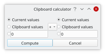
Clipboard calculator
Figure 10:Clipboard calculator.
The clipboard calculator allows you to perform arithmetic operations with the values stored in the clipboard, the current reaction rates or a fixed value that you can enter in this dialog.
The result of the operation replaces the current flux values.